by Luigi Mariani and Franco Zavatti
The reference dataset
Europe is the world region with the longest time series of instrumental data due to the fact that the first meteorological instruments (thermometer, pluviometer, evaporimeter and barometer) were invented by some scientists of the Galilean school (Accademia del Cimento). In this highly original scientific context flourished for the first time the idea of spreading meteorological instruments at the European level to promote an observing network that would operate in a coordinated manner (Iafrate, 2008). The availability of very long time series is quite interesting for historical and climatological purposes although the homogeneity of such series is negatively affected by changes in:
- measurement units
- observational standards (e.g.: time of observation)
- location of instruments
- intensity of urban effects (intensity of the urban heat island UHI).
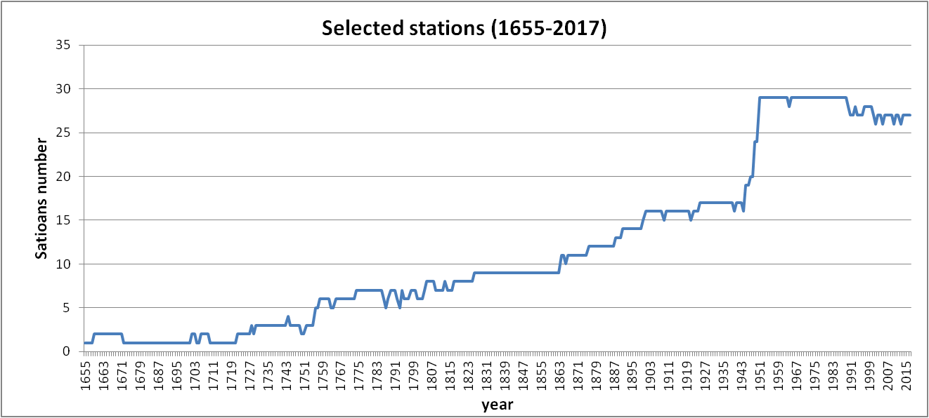
The data of European stations shown in Figure 1 (in Table 1 is reported the list of selected stations with the meaning of the acronyms) were gathered with the aim of organizing an easily updatable dataset which allows us to give an overview of the trend of European climate over the long time periods covered by instrumental data.
The final dataset resumed in the file EUROPA_TD_da_1655_DATI e RISULTATI.xls began in 1655 which is just the beginning of the Florentine Galileo series data (Camuffo and Bertolin, 2012). The central England time series CET (MetOffice – Hadley Centre, 2016) was added from year 1659 and gradually other stations have joined, at first coming from historical observatories (Camuffo and Jones, 2002) and then from current operational networks. The most recent data come from either the web site Rimfrost (2016) and from the web sites of Meteofrance, ECA&D and MeteoSwiss.
All data sources are reported in the data file and are highlighted by different colors.
Data processing and final product
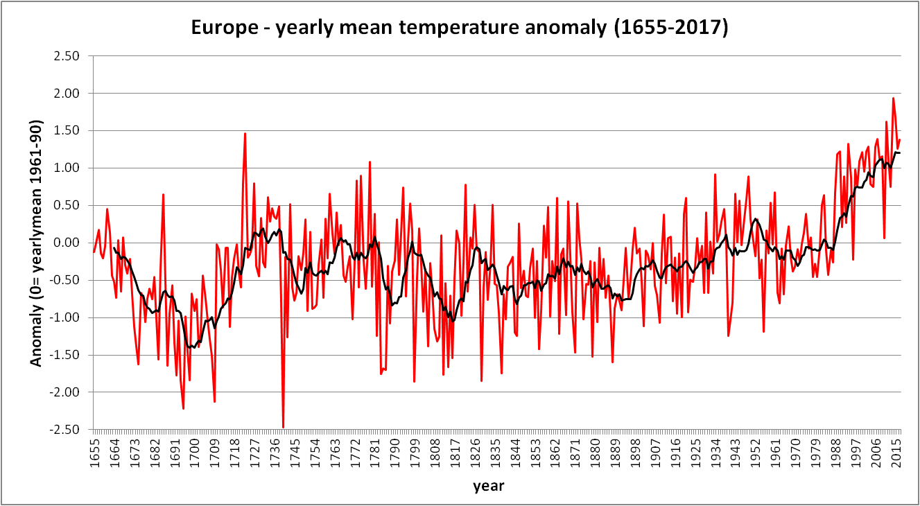
In order to obtain a representative areal average, the data of each station were converted into anomalies with respect to the average temperature 1961-1990 of the station itself. The final product is given by the diagram of the yearly average European temperature anomaly for the period 1655-2015. The final results are freely available in the excel file EUROPA_TD_da_1655_DATI and RISULTATI.xls.
Data quality
A constant problem for people that aim to rebuild the behavior of European air temperature at synoptic scale is the influence of the UHI, a micro-meteorological phenomenon which is often present in a densely populated areas such as Europe where meteorological measurements began in geophysical observatories often placed at the center of large urban areas. The weight of the UHI is absent only for rural measurement stations or high altitude stations (Sonneblick, Gran San Bernardo).
In order to evaluate the weight of the UHI on the time series 1655-2015, it may be helpful to look at the diagram of deviance (sum of the squared deviations from the mean) of the temperature anomalies, represented in Figure 4. The value of the deviance:
- shows a weak increase since the mid-1850 to date, moving from average values of 4.7 for the period 1851-1900 to the average value of 6.15 for the period 1951-2015. Note that the period from 1851 to the present day is marked by an increase in the number of stations that increase the representativeness of the selected network. This could explain the increase of the deviance.
- is mostly stable from the 50s of the twentieth century, when the number of stations becomes almost stationary (figure 2). This could be the result of the substantial stability of the UHI for the selected network. However this statement has some limitations because the deviance is not only affected by UHI. For example with a zonal circulation regime (Atlantic atmospheric currents driven by a robust anticyclone over the Mediterranean and by a low pressure belt on the Northern Sea) the deviance could be more pronounced than with a blocking regime more favorable to latitudinal exchanges. Moreover the different factors acting on the deviance could counter-balance among them.
I’d like also to point out that the three Spanish stations of Salamanca, Navaracerrada and Cadiz have a very low correlation with the Central England series CET, which is not evident for the other stations of the dataset. I think that in future it will be necessary a deeper reflection on the Spanish reference stations.
Results
The selected time series covers a very long period which contains the present warming period (1850 – today) and a substantial part of the Little Ice Age (LIA).
The anomalies of the diagram (Figure 3) are the result of three types of phenomena:
- A warming trend associated with the exit from the LIA. The diagram in Figure 3 shows that we passed by values up to -2.5 ° C below the average 1961-90 (value of 1740, which is the coldest year of the entire series) at current values of 2 ° C above the average itself (value of 2014 which is the hottest year of the series).
- A very strong interannual variability that is one of the “key features” of the European climate. This variability is the result of the changes in frequency and persistence of various circulation types affecting our continent and European citizens should in any case consider this phenomenon when performing choices affected by climate (agriculture, energy, transport, health, etc.)
- A multi-yearly cyclicity (with a 38 years period on the average) that is the result of the cyclical variation of ocean temperatures described by the AMO index. When AMO is in a positive phase and the ocean is warm even European temperatures are higher and when AMO passes in negative phase and the ocean turns cold European temperatures become lower. Note that the transition from the AMO cold phase to warm one is triggered by some years of Atlantic atmospheric circulation (westerlies) very intense as shown by the positive value of winter NAO (NAOI). The powerfulness of the AMO is quite relevant. Note for example that in the cold phase that goes from late ‘50s to 1987, European temperatures have been run down to values close to those of period 1900 – 1930.
The visual analysis of the European average temperature anomaly (Figure 3) shows that the inter-annual variability is not significantly increased compared to the past. This is consistent with results of Anderson and Kotinski (2010 and 2016) that working on 6092 monthly global monthly series with at least 90 years of data from the GHCN dataset and highlighted a decrease in the average temperature inter-annual variability for the analysed period (1900-2013).
Similarly, the visual analysis of the deviance diagram (figure 4) shows that spatial variability is not significantly increased compared to the past and appears roughly stationary since the middle of the nineteenth century. This leads to the belief that frequency distribution in the various spatial scales of the circulatory structures responsible for such variability has not substantially changed over time.
How to cite this dataset
The dataset of mean temperature anomalies for Europe in its version updated to 2015 was among the databases of weather data and biological proxies used to analyze the mean climatic cycles that affect European climate (Mariani and Zavatti, 2017). Please refer to this job while use these data for research purposes.
Acknowledgments
I’d like to thank Costantino Sigismondi and Franco Zavatti for the critical review of the text.
References
- Anderson A. e Kostinski A., 2010 Reversible Record Breaking and Variability – Temperature Distributions across the Globe, Journal of applied meteorology and climatology, vol. 49, 1681-1691, DOI: 10.1175/2010JAMC2407.1
- Anderson A., Kostinski A., 2016. Temperature variability and early clustering of record-breaking events, Theor Appl Climatol (2016) 124:825–833, DOI 10.1007/s00704-015-1455-5
- Camuffo D. and Bartolin C., 2012. The earliest temperature observations in the world: The Medici Network (1654-1670), Climatic Change 111(2):335-363 · July 2012.
- Camuffo D. and Jones P.D. 2002. Improved Understanding of Past Climatic Variability from Early Daily European Instrumental Sources. Kluwer Academic Publisher, http://www.wkap.nl/prod/b/1-4020-0556-3 (site visited at 7 January 2016).
- Iafrate L., 2008. Fede e Scienza: un incontro proficuo. Origini e sviluppo della meteorologia fino agli inizi del ‘900. Roma: Ateneo Pontificio Regina Apostolorum (Scienza e Fede, Saggi: 4). ISBN: 978-88-89174-52-4.
- Mariani L., Zavatti F., 2017. Multi-scale approach to Euro-Atlantic climatic cycles based on phenological time series air temperatures and circulation indexes, Science of the Total Environment 593–594 (2017) 253–262
- Metoffice – Hadley Centre, 2015. Hadley Centre Central England Temperature (HadCET) dataset, http://www.metoffice.gov.uk/hadobs/hadcet/ (site visited at 7 January 2016).
Rimfrost – Data on global weather stations, http://www.rimfrost.no/ (site visited at 7 January 2016).


| n | nome | acronimo | altezza | latitudine | longitudine |
| 1 | Central_England_Temperature | CET | 100 | -1.00 | 52.00 |
| 2 | SONNBLICK | SBLI | 3109 | 12.95 | 47.05 |
| 3 | HAMBURG Fuhlsbuttel | HAMB | 11 | 9.59 | 53.38 |
| 4 | NAVARACERRADA | NAVA | 1890 | -3.59 | 40.46 |
| 5 | SALAMANCA | SALA | 590 | -5.28 | 40.56 |
| 6 | BOURGES | BOUR | 166 | 2.37 | 47.07 |
| 7 | MONT-AIGOUAL | MAIG | 1567 | 3.35 | 44.07 |
| 8 | RENNES | RENN | 36 | 1.44 | 48.04 |
| 9 | STRASBOURG | STRB | 154 | 7.63 | 48.55 |
| 10 | TOULOUSE (BLAGNAC) | TOUL | 151 | 1.22 | 43.37 |
| 11 | UPPSALA | UPPS | 20 | 17.38 | 59.51 |
| 12 | STOCCOLMA | STOC | 20 | 18.04 | 59.19 |
| 13 | BERLIN TEMPELHOF | BERL | 34 | 13.24 | 52.31 |
| 14 | PARIS MONTSOURIS | PARI | 75 | 2.34 | 48.82 |
| 15 | SAN PIETROBURBO | SPIE | 20 | 30.19 | 59.56 |
| 16 | FRANKFURT AM | FFUR | 110 | 8.41 | 50.07 |
| 17 | KREMSMUENSTER | KREM | 384 | 14.08 | 48.03 |
| 18 | CBT_BELGIO-BRUXELLES | BRUX | 100 | 4.60 | 50.51 |
| 19 | DE-BILT | DEBI | 15 | 5.18 | 52.10 |
| 20 | POPRAD TATRY | POPR | 695 | 20.25 | 49.07 |
| 21 | WADDINGTON (LINCOLN) | WADD | 70 | 0.52 | 53.17 |
| 22 | BASEL-BINNINGEN | BASL | 316 | 7.60 | 47.60 |
| 23 | VERONA VILLAFRANCA | VERO | 68 | 10.52 | 45.23 |
| 24 | CAGLIARI ELMAS | CAGL | 2 | 9.13 | 39.14 |
| 25 | BRINDISI | BRIN | 10 | 17.56 | 40.38 |
| 26 | PADOVA | PADO | 10 | 11.52 | 45.24 |
| 27 | CADICE | CADI | 10 | -6.17 | 36.31 |
| 28 | COL DU GRAN ST_BERNARD | CGSB | 2472 | 7.17 | 45.87 |
| 29 | FIRENZE | FIRE | 40 | 11.20 | 43.81 |
